
2020 Edition

Winners of the 1st Edition (2020)
After having evaluated the proposals of the participant teams, the winners of the challenge are:
- Ramon Vallès
- ATARI
- STC (team 2)
We wish you the best of luck for the final!
We would also like to recognize the work done by the other teams that made it to reach phase 2 of the challenge:
- NETCOM
- NET INTELS
1. Presentation
This challenge was promoted by Universitat Pompeu Fabra (UPF) and was part of the ITU Artificial Intelligence/Machine Learning in 5G Challenge. Participation was open to ITU members and any individual from an ITU Member State. “Participants” were individuals or companies that participate in the ITU AI/ML in 5G Challenge, providing solutions to problem sets of the Challenge. This challenge was open to two categories of participants: student and professional.
Presentation of the problem statement:
- Video introducing the problem statement and the dataset
- Presentation (in pdf) introducing the problem statement and the dataset
2. Background
Next-generation IEEE 802.11 wireless local area networks (WLANs) are called to face the challenge of providing high performance under complex situations, e.g., to provide high throughput in massively crowded deployments where multiple devices coexist within the same area. To address the performance challenges posed by the requirements derived from novel use cases, one of the features receiving more attention is Channel Bonding (CB) [1, 2], whereby multiple frequency channels can be bonded with the aim of increasing the bandwidth of a given transmission, thus potentially improving the throughput.
Since its introduction to the 802.11n amendment, where up to two basic channels of 20 MHz could be bonded to form a single one of 40 MHz, the specification on CB has evolved and currently allows for channel widths of 160 MHz. However, using wider channels entails spreading the transmit power over the selected channel width, which can potentially affect the data rate used for the transmission, and the capabilities of the receiver on decoding data successfully. Moreover, the potential gains of CB in crowded deployments is further hindered because of the multiple inter-BSS interactions, which may provoke contention based on the global channel scheme (i.e., the set of channels allocated to each BSS). In particular, CB in dense deployments is a problem with a combinatorial action space.
To address the CB problem in WLANs, we propose the application of Machine Learning (e.g., Deep Learning) to predict the performance of an OBSS where different combinations of channel schemes are allocated to the different BSSs. The main purpose is, therefore, to predict the throughput that a BSS would obtain according to the data extracted from simulated deployments generated based on different random parameters, including channel allocation, location of nodes, and number of STAs per BSS.
Performance prediction in WLANs can be used to optimize the planning phase of a given deployment or improve the performance during the operation of a WLAN.
3. Data set
The entire data set can be downloaded here.
NOTE: The data set is completely open, free of charge, accessible, and reusable.
Training data set:
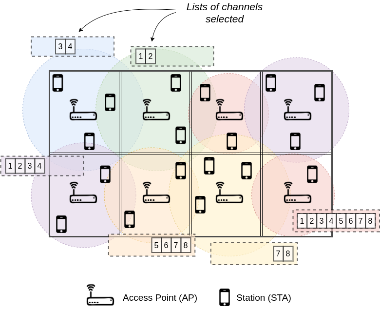
The assets provided comprise both training and validation data sets of CB in IEEE 802.11 WLANs. Each of the data set partitions includes two different enterprise-like scenarios, where a different fixed number of BSSs coexist in the same area. Scenario 1 is composed of 12 APs, each one with 10 to 20 associated STAs, while Scenario 2 has 8 APs with 5 to 10 STAs per AP. Each of the scenarios is reproduced in random deployments for three different map sizes. The summary of the provided deployments is as follows:
-
Scenario 1 (12 APs, 10-20 STAs):
-
Scenario 1a (map size = 80 x 60 m): 50 random deployments
-
Scenario 1b (map size = 70 x 50 m): 50 random deployments
-
Scenario 1c (map size = 60 x 40 m): 50 random deployments
-
-
Scenario 2 (8 APs, 5-10 STAs):
-
Scenario 2a (map size = 60 x 40 m): 50 random deployments
-
Scenario 2b (map size = 50 x 30 m): 50 random deployments
-
Scenario 2c (map size = 40 x 20 m): 50 random deployments
-
Test data set:
Similarly to the training data set, the test data set includes a set of deployments and random scenarios depicting multiple CB configurations in WLANs. In this case, 4 different scenarios are considered according to the number of APs (4, 6, 8, and 10 APs). Each scenario has been represented with multiple random deployments (in total, 50 deployments per each scenario), where the number of STAs, the location of STAs, and the CB configuration have been randomly chosen. The test data set is structured as follows:
- Scenario 1 (test_1): 50 random deployments in a map of size 80x60m
- Scenario 2 (test_2): 50 random deployments in a map of size 80x60m
- Scenario 3 (test_3): 50 random deployments in a map of size 80x60m
- Scenario 4 (test_4): 50 random deployments in a map of size 80x60m
The test data set includes the same features as provided in the training data set except the throughput, which is the prediction goal of this challenge.
Apart from that, the output generated by the simulator has been processed for each type of scenario. According to this, the information extracted from each simulation (interference map, RSSI, SINR, and airtime) has been provided in separated files
Overview of the data set:
Two types of files are provided:
- Nodes' input files: input files defining the network deployments used to run the simulator
- Output Komondor: output generated by the simulator after running the nodes' input file
To train an ML model, participants should use both input features (deployment characteristics) and labels (performance). The features can be obtained from both nodes' input files and Komondor's output. Apart from the performance labels (throughput and airtime), the output of the simulator provides the RSSI list and the interference map (further described below).
Input features:
-
Deployment characteristics (provided in input nodes files): labels and locations of the nodes and the selected channel scheme. Input files contain other static information (e.g., CW size) that is not recommended to be used for training.
-
RSSI list (provided in output files): RSSI in dBm that each device receives from its AP. Each row represents a BSS.
-
Interference map (provided in output files): inter-BSS interference sensed from each AP in dBm. Each row represents the signal strength that each AP receives from all the other APs.
-
Signal-to-Interference-plus-Noise Ratio (provided in output files): average SINR experienced by each device during packet receptions. The SINR values in APs are marked as Inf because we focus on the DL traffic sent to STAs.
Output labels:
-
Per-STA throughput (provided in output files): average throughput experienced by each STA at the end of the simulation, being the throughput of the AP the aggregate throughput of the BSS (i.e., the sum of all the individual throughput allocated to each STA in the BSS).
-
Airtime per channel (provided in output files): percentage of time each BSS occupies each of the assigned channels. E.g., if a given BSS transmits during 80% of the time in both channels 3 and 4, the airtime will be provided as {80, 80}. Important: the airtime is an auxiliary label that seeks to provide a further understanding of the interactions taking place in each simulated deployment.
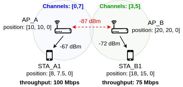
Example of a data set entry:
For the sake of illustration, here we show a simplified data set entry.
-
Input node files (contains the characteristics of the deployment). The most important features are shown in the following table.
|
node_code |
node_type (0:AP, 1:STA) |
wlan_ code |
x |
y |
z |
primary_channel |
min_channel_allowed |
max_channel_allowed |
|
AP_A |
0 |
A |
10 |
10 |
0 |
0 |
0 |
7 |
|
STA_A1 |
1 |
A |
8 |
7.5 |
0 |
0 |
0 |
7 |
|
AP_B |
0 |
B |
20 |
20 |
0 |
3 |
3 |
5 |
|
STA_B1 |
1 |
B |
18 |
15 |
0 |
3 |
3 |
5 |
* Notice that input files include other static information such as the channel bonding model, the minimum Contention Window (CW), etc. This information is recommended to be ignored for training your algorithm.
-
Simulation output files (includes labels and features). Information is provided in the following order:
- Per-STA throughput (in Mbps): {100, 100, 75, 75}
* In this case, there is only one STA per BSS, so the aggregate throughput is the same as the throughput obtained by STAs. The order of appearance matches the indicated in the nodes' input files. The size of this array is [#APs + #STAs].
- Airtime per BSS per channel (in %): {80, 80, 80, 50, 50, 50, 50, 50; 50, 50, 50}
* Note that information is shown for each BSS (separated by a semicolon) and only for the set of selected channels. Thus, the size of this array is dynamic.
- RSSI list (in dBm): {Inf, -67, Inf, -72}
* Notice that APs are also included in the list, but the RSSI received from themselves is marked as ‘Inf’. The size of this array is [#APs, #STAs].
- Interference map (in dBm):
{Inf, -87;
-87, Inf}
* Notice that each AP receives an Infinite amount of power from itself. The size of this array is [#APs, #APs].
- SINR (in dB): {Inf, 20.12, Inf, 32.89}
The output results for all the deployments of each scenario is provided in the same file (e.g., “script_output_sce1a.txt”). Each deployment is introduced with the following header:
KOMONDOR SIMULATION ‘sim_input_nodes_sce1a_deployment00.csv’ (seed 1992),
which includes the name of the input nodes file used to conduct the simulation (in this case, ‘sim_input_nodes_sce1a_deployment00.csv’) and the random seed.
How was the data set generated?
To generate the data set, we have used the Komondor simulator (https://github.com/wn-upf/Komondor, Commit: 96f440901966c6dacb138532b2631d5068627c0d), an IEEE 802.11ax-oriented network simulator developed at the UPF. Komondor has been validated against ns-3 [3] and includes novel functionalities such as channel bonding and spatial reuse.
The main parameters used to conduct the simulations are as follows:
- Simulation duration: 10 seconds
- Downlink UDP traffic (full buffer)
- The traffic of a BSS is uniformly spread among STAs
- Random channel allocation
- Random number of STAs per BSS
- Location of APs is fixed at the center of each cell
- The location of STAs is randomly selected around the AP
- A dynamic channel bonding policy has been applied, whereby nodes attempt to transmit over the widest possible channel
4. Submission guidelines of the 1st edition
The submission was split into two phases:
- Phase 1: submit predictions of the throughput of each AP of the test deployments.
- Phase 2: submit code and documentation explaining your solution.
Evaluation criteria
-
Participants must use the provided data set to train a machine learning algorithm.
-
The output of the ML algorithm should be able to predict the performance obtained in a new network deployment. In particular, the expected throughput of each BSS in the deployment must be provided.
-
The choice of the ML approach is decided by each participant (neural network, linear regression, decision tree, etc.).
-
A test data set will be provided to evaluate the performance of the proposed algorithms.
-
The evaluation of the proposed algorithms will be based on the average squared-root error obtained along with all the predictions compared to the actual result in each type of deployment.
-
The winners will be invited to publish the results in an academic publication.
Phase 1
- Participants will submit their predictions of the throughput in each of the deployments of the test data set.
- In particular, the solution must be, for each deployment, an array of the throughput obtained by every AP.
- For instance, in a deployment with 4 APs, the output should be {throughput_AP1, throughput_AP2, throughput_AP3, throughput_AP4}
- Optionally, participants can provide the throughput obtained by every device, including STAs. Notice that the throughput of an AP is the aggregate throughput of all its associated STAs.
- The throughput of each AP/device must be in Mbps.
- The solution must be separated into 4 different folders (one for each of the 4 test scenarios).
- In each of the folders, there should be 50 different files (one for each of the 50 deployments) including the throughput arrays.
- The format of the files is preferable to be .csv (.txt will also be accepted).
- Detailed solution structure:
- Folder 1 (test scenario 1 - 4 APs):
- File 1 ("throughput_1.csv"): {throughput_AP1, ..., throughput_AP4}
- ...
- File 50 ("throughput_50.csv"): {throughput_AP1, ..., throughput_AP4}
- Folder 2 (test scenario 2 - 6 APs):
- File 1 ("throughput_1.csv"): {throughput_AP1, ..., throughput_AP6}
- ...
- File 50 ("throughput_50.csv"): {throughput_AP1, ..., throughput_AP6}
- Folder 3 (test scenario 3 - 8 APs):
- File 1 ("throughput_1.csv"): {throughput_AP1, ..., throughput_AP8}
- ...
- File 50 ("throughput_50.csv"): {throughput_AP1, ..., throughput_AP8}
- Folder 4 (test scenario 4 - 10 APs):
- File 1 ("throughput_1.csv"): {throughput_AP1, ..., throughput_AP10}
- ...
- File 50 ("throughput_50.csv"): {throughput_AP1, ..., throughput_AP10}
- Folder 1 (test scenario 1 - 4 APs):
Phase 2
- Participants will submit the code used* to generate their predictions. This part of the submission is divided into:
- Source code used in the challenge
- Documentation / How-to-use guide
*It is strongly recommended to post the code on Github and make it publicly available for the sake of transparency and reproducibility.
- A report describing their solution will also be submitted (4-6 pages). The report must include:
- The motivation of the considered approach
- A description of the proposed approach
- Besides, it is recommendable to include the insights and conclusions obtained during the entire research activity. For that, participants can use figures to illustrate the performance of their solution at both training and test data sets.
------------------------------------------------------------
Contact
Francesc Wilhelmi ([email protected])
Boris Bellalta ([email protected])
ITU AI Challenge committee ([email protected])
References
[1] Barrachina-Muñoz, S., Wilhelmi, F., & Bellalta, B. (2019). Dynamic channel bonding in spatially distributed high-density WLANs. IEEE Transactions on Mobile Computing.
[2] Barrachina-Muñoz, S., Wilhelmi, F., & Bellalta, B. (2019). To overlap or not to overlap: Enabling channel bonding in high-density WLANs. Computer Networks, 152, 40-53.
[3] Barrachina-Muñoz, S., Wilhelmi, F., Selinis, I., & Bellalta, B. (2019, April). Komondor: a wireless network simulator for next-generation high-density WLANs. In 2019 Wireless Days (WD) (pp. 1-8). IEEE.