Courses
Basic Syntax
Data in R can be stores in variables (also referred as RObjects) of different data types. The most frequently are vectors, lists, matrices, factors and data frames. The data contained can be of class:
- Logical: TRUE, FALSE
- Numeric: 10, 12.9
- Integer: 10L
- Complex: 15 + 3i
- Character: "Hello", 'Hello', "14"
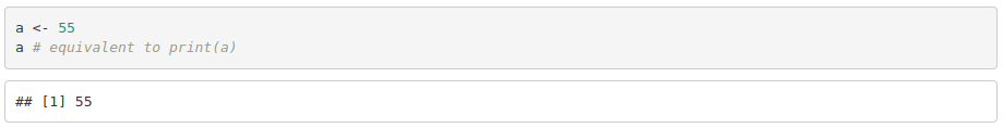
To assign values to variables we use " <- ", for instance
When a variable or a vector class is unkwown, use the function class(variable_name).
Vectors
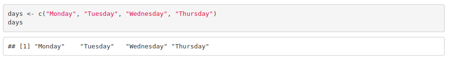
Vectors with multiple elements are created using c(), a function to combine elements.
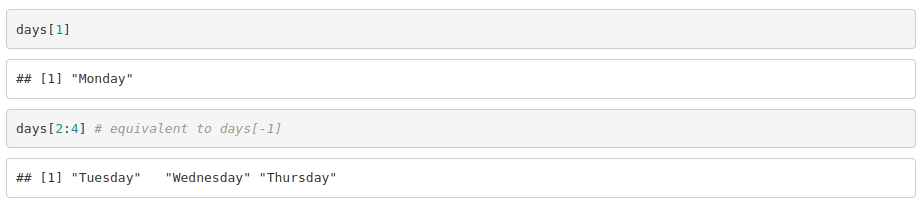
To access the elements of a vector:
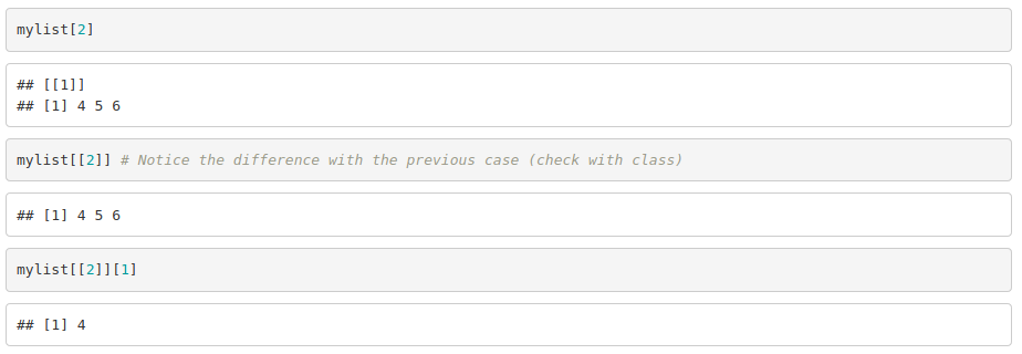
Lists
Lists are created using list() and it can contain different types of elements such as vectors, functions and even further lists.

To access the elements:
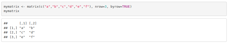
Matrices
To create them we use matrix(vector, nrow, ncol, byrow). For instance:
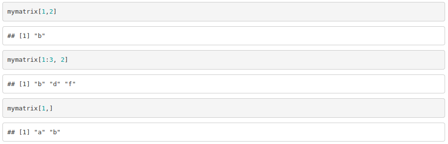
To access to the elements of a matrix, we need to specify the row (or rows) followed by the column (or columns) of interest.
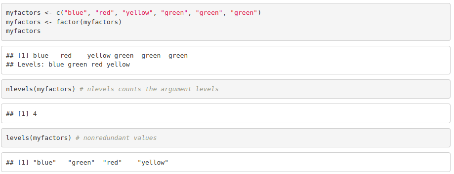
Factors
Factors are created from a vector using factor(vector). It stores the vector and its unique elements. Each level corresponds to a unique element.
Data Frames
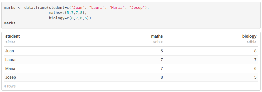
Unlike matrices, they can store different types of elements. They are generated using data.frame(). When importing a table from a .txt or .xlsx file, R will automatically read it into a data frame object.
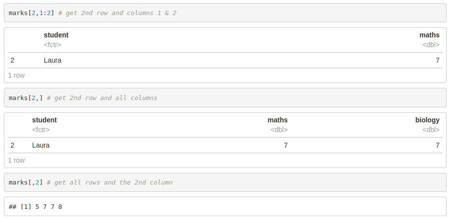
We access data frames the same way we do with matrices
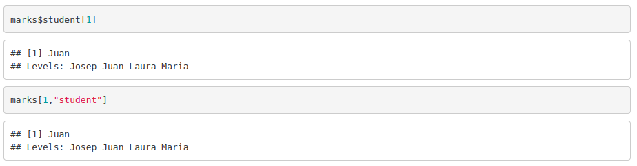
Additionally, you can access to columns by its name:
Operators
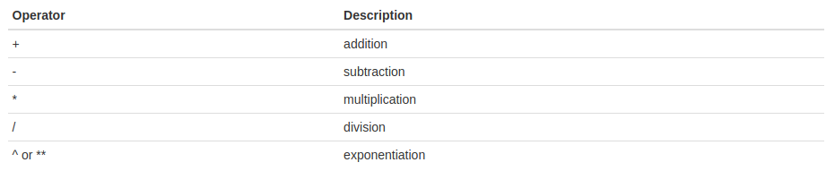
Arithmetic operators:
Relational and logical operators:
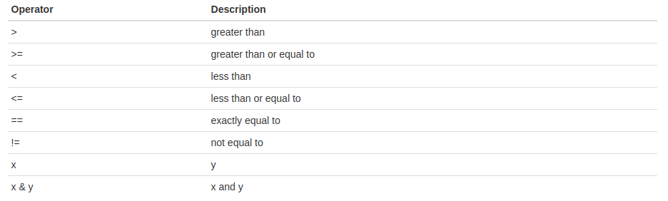
These operators compare each element of the first vector to the corresponding element of the second vector and return a boolean value (TRUE or FALSE).
Built-in functions
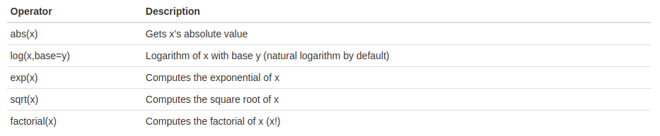
- Math functions
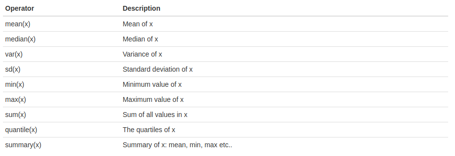
- Statistical operators
- Other functions of interest:
In order to import data in the R global environment, you can use read.table, a function that imports text or comma-separated files into a data frame. read.csv and read.delim are some of the other available functions for this purpose. However, they only differ in the default arguments (header, separator,…).
You can also use the global environment menu. Just look for the “Import Dataset” button.
To export a data frame from the R global environment to a text or comma-separated file, you can use write.table and write.csv among others. Basically, you need to specify which is the data frame variable that you need to save and the filename. Additional arguments can be given to determine the field separator, among others.

- Installing and using packages: We use the following command to install the library

Then, to load the package and use it:

How to create use-defined functions?
To write a function we need to take into account:
- Function name, to identify the function in the environment and to call it.
- Argument, to set the inputs. These are optional and can have default values.
- Body, containing the statements that R will execute.
- Return value.
The syntax is as following:
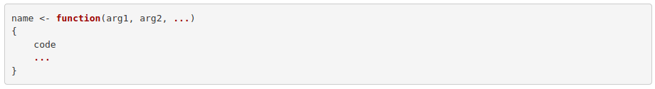
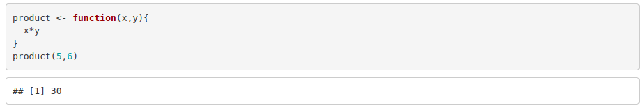
An example to calculate the product of two numbers:
Control Structures
Sometimes we need to execute different blocks of code depending on a particular condition, or we need to execute it several times until a condition is fulfilled. To do so in R, we can use the following structures:
- if statement: R will execute the code only if the condition is TRUE.

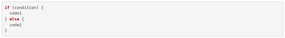
- if ... else statement: If the condition is true, code1 will be executed. Else, R will execute code2.
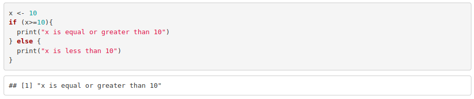
For example:
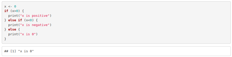
If there are more than two alternatives:
- while loop: R will execute the code in the while loop until a condition is fulfilled.

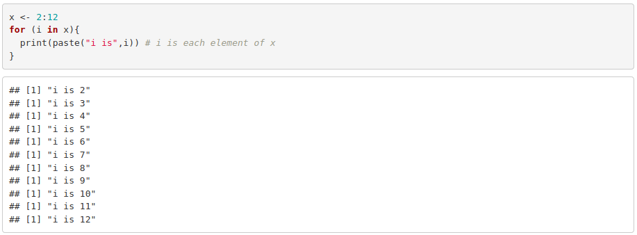
- for loop: In a for loop, the code will be executed for each element of a vector or given a number of repetitions.
- Alternatives to R loops: the apply() family
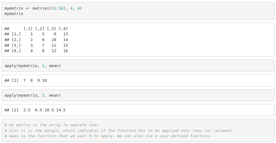
The “apply family” consists of a set of functions to manipulate different types of data (arrays, lists, data frames) avoiding the explicit use of for loops. They are less intuitive than the latter but more efficient.
- apply() acts on arrays or matrices
- lapply() acts on vectors and returns the result in the form of a list
- sapply() works as lapply() but returns a vector
For example:
Plotting in R with ggplot
ggplot2 is based on the idea that you can build all graphs based on the same components:
- a data frame
- the aesthetics: x, y and any color, size, shape, fill… associated to a variable in the data frame.
- the geometry: type of plot (scatterplot, barplot, density plot, histogram..)
The basic syntax is:

Some notes about it:
- ggplot() begins the plot and is the function where we normally specify the data frame whose variables we want to plot.
- aes() is the function to specify the aesthetics. As we have already specified the data frame, we do not need to do data_frame$var_name when defining the axes. Just do x=var1, y=var2, color=var3, …
- aes() can be set in ggplot() or directly in the geometry function. (geom_point(), geom_line(), geom_histogram()).
- Geometry functions build on ggplot() and thus, they do not work by themselves.
- We can use multiple geometry functions in the same plot, just by adding them up.
There is a public ggplot2 cheat sheet, which is very useful for checking the syntax and to see the wide range of options that the package provides.
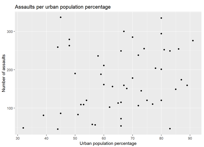
Now, let’s make some plots using ggplot2 using the USArrests dataset included in R ( to use it just write data("USArrests") ). First of all, you need to upload the library:

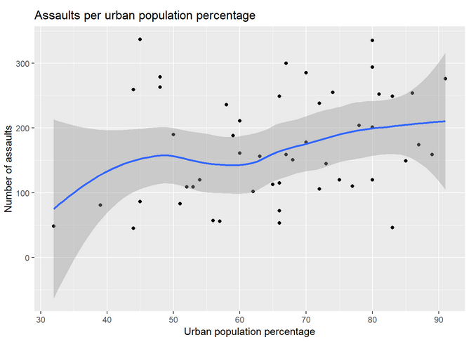
Next, to make a scatterplot of the assaults per urban population:

The plot should look like this:
Let’s adjust a curve to the data by adding geom_smooth():
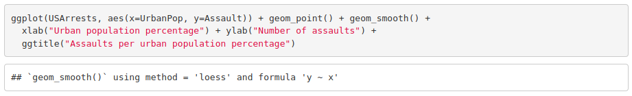
Which should look like this:
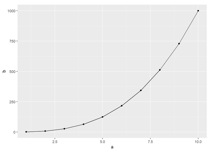
The line plot with ggplot is done with this command:

And it should look like this:
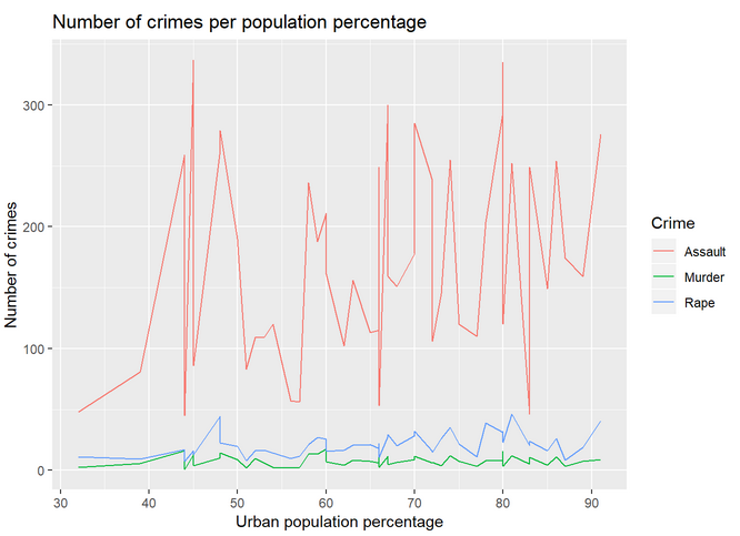
Let’s plot the lines for all the variables of USArrests. To do so, we need to modify the data frame so that we have a column with the type of crime and another column with the number of crimes (instead of a column per crime). By doing so, we are transforming the data from wide to long format. Once done that, we just need to specify in the aesthetics that we want to color the lines by crime. See:
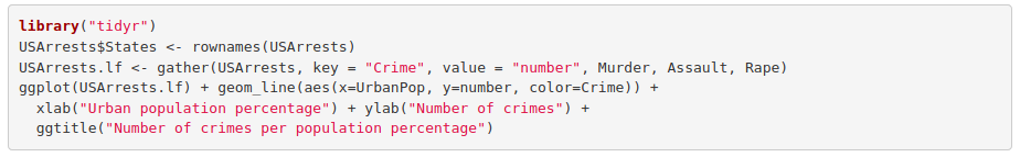
The lines should look like the following plot:
And to plot the bar chart of the same data:

And its plot:

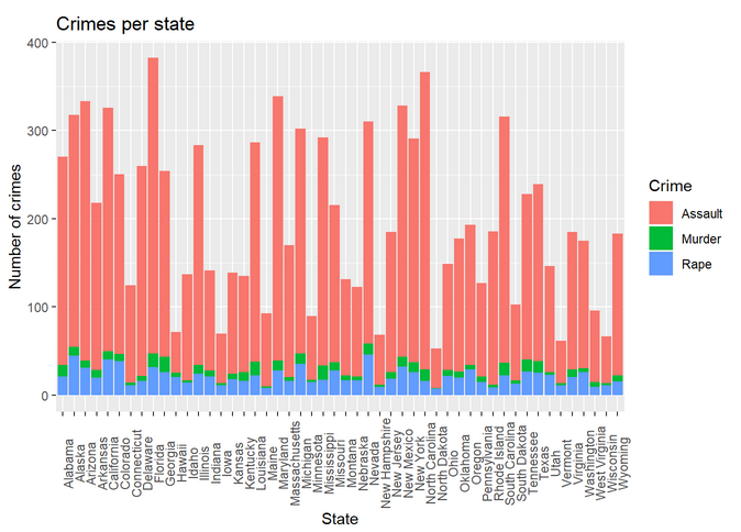
Let’s represent in the same bar plot the number of each crime. Here we also need the long format data frame to specify that we want different filling colors per crime.
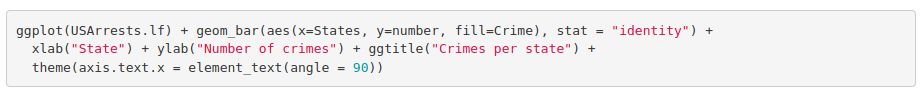
The corresponding plot is:
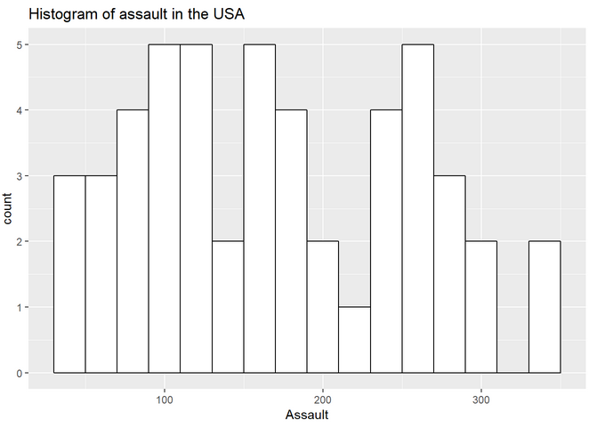
Histogram:

The histogram with larger bin size and no color:
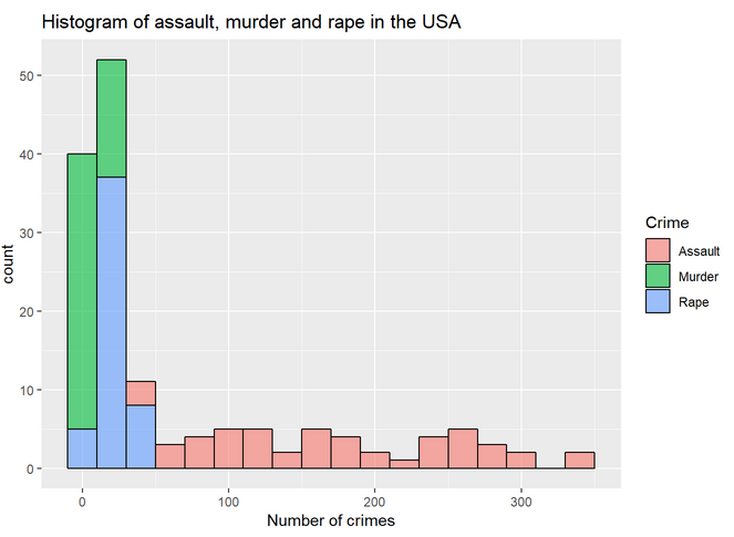
Again, we represent in the same histogram all the crimes:

Since we use "fill = Crimes", we will have the histogram represented with distinct colors for each crime:
We also can plot boxplots with ggplot:

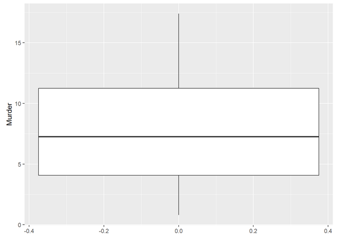
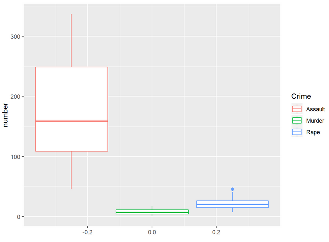
Finally, let’s make a boxplot with all the crimes:

Hypothesis testing
Usually, when we collect data from an experiment or download it from a public database we want to test if a hypothesis is true. Statistical tests can be parametric or non-parametric. Parametric tests assume:
- Data is normally distributed
- Homoscedasticity (variance homogeneity)
- Data is independent (there is no correlation)
1. Does our data follow a normal distribution?
The central limit theorem determines that distributions of sufficiently large samples (>30) tend to normality. Because of that, sometimes people do not assess the normality of their data. For other cases (or if you just want to make sure), normality can be assessed by visual inspection or by significance tests.
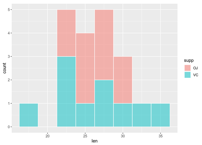
Let’s see some examples using the ToothGrowth dataset. Visual inspection can be done using histograms/density plots or qqplots.

The histogram shows:
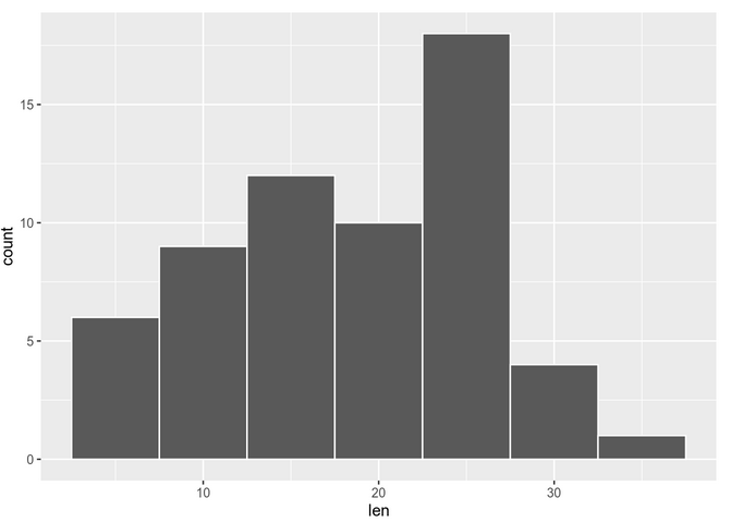
We can also check with a qq-plot:


In theory we should be checking normality by group. To simplify, we are going to be comparing the same dose of Vitamin D (2 mg/day) for the two delivery methods. So, for instance:
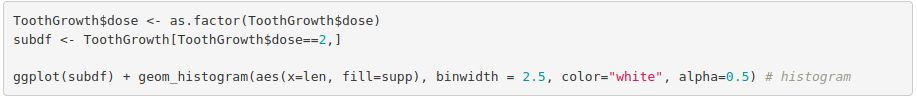

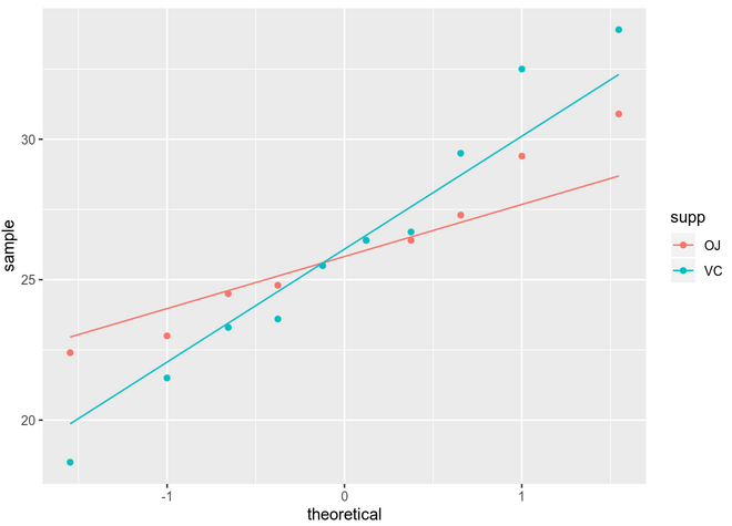
You can see that assessing normality can be quite subjective if we just use visual methods. Some of the mostly used significance tests to objectively test normality are: Kolmogorov-Smirnov (K-S) and Shapiro-Wilk’s test (better power).
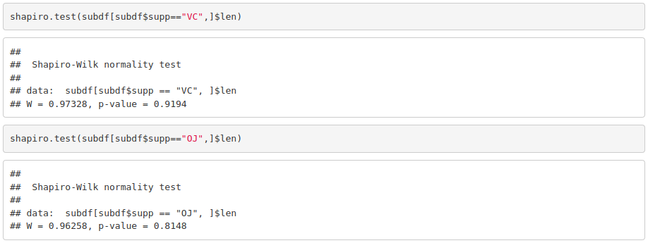
Because the obtained p-value is greater than 0.05, we cannot reject the null hypothesis stating that our data is normal.
2. Is the data homocedastic?
If the data is normal, then we check if variances in both groups being compared is also equivalent. One way to check that is using the F test, which is based on the variances ratio.
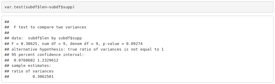
Again, a p-value of 0.09274 is not enough to reject the null hypothesis that tells us that variances are equivalent.
Apply a chosen statistical set
Once normality and homoscedasticity are checked, we choose the appropriate statistical test. In this case, as we have normal and homoscedastic data we can use a parametric test –> t test.
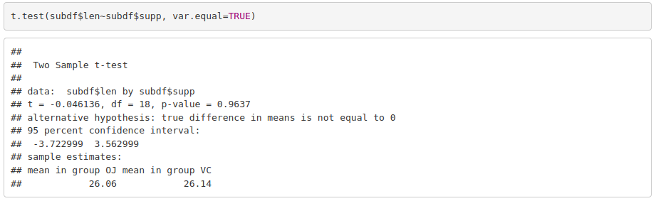
For a dose of 2 mg/day, the response in the guinea pigs does not depend on the delivery method.
R Markdown
Markdown is a formatting language where plain text documents are converted into rich text files with different formats (word, pdf and originally HTML). It can have code and figures embedded. It can be used to generate high quality reproducible reports but also simpler things such as README files, forum questions…
R Markdown not only allows saving code but also executing it directly in the file, which is a huge time saver. The document in which we work is in .Rmd format, which combines R code with markdown. When we knit the file, knitr transforms it into a classic markdown file (.md) by automatically writing the code and its output in the proper format. The finished pdf, word or HTML is then generated by pandoc. Do not worry, this is all done internally when clicking knit.
We need to install the rmarkdown package as follows

The formatting syntax is really easy to learn. You can take a look to the reference guide.
Good Practices
So far, we have only programmed very small chunks of code. Whenever you start using R for your projects it is recommended that you follow some good practice rules:
- Write your code in source files (.R files) and save changes frequently –> In RStudio: Cntrl + Shift + N.
- Add comments to your code. You might know what it does now, but if you go back to it later, you will thank yourself for putting comments. –> Just use # at the beginning of the sentence.
- For if…else, for loops, while loops, functions …, use new lines and proper indentation. Make it as structured and visual as possible.
- Keep function and variable names simple. They should be short but also self-explanatory.
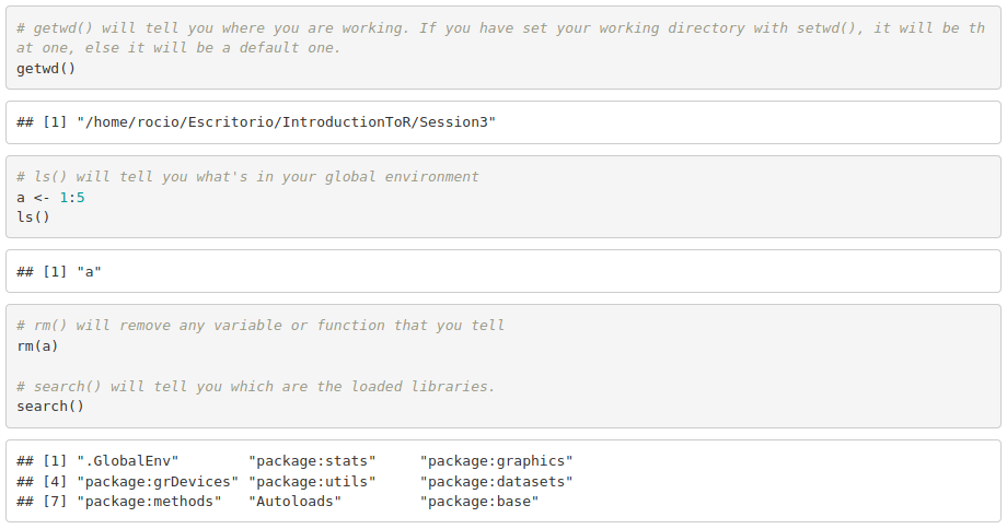
- Set the working directory (setwd()) to have access to all the files in that directory and know where you are saving new files.
For computational efficiency of large scripts/functions, bare in mind:
- Always try to avoid loops. Hint: Can you use a function from the apply() family to avoid it?
- Do NOT grow objects within loops. Instead of adding a new element to a vector in each iteration, it is preferable to substitute the corresponding element of an empty vector (with NAs or 0s).
- Instead of using if…else for filtering data frames, can you use subsetting?
Some miscellaneous useful functions. Try: